How To Detect and Handle Outliers in Data Mining [10 Methods]

Outliers are those things that you will always have present in your data mining, data analysis, data science project. Indeed, there are those data points that significantly differ from the rest of the pack. In this article, I will be giving you insights on what are outliers, before showing you a couple of techniques on how you can handle them using python.

What are outliers?

In data mining, outliers are data points that deviate significantly, or in simpler terms are “far away”, from the rest of the data point.  

Outliers can be in both the univariate and multivariate forms. Univariate outliers are observations that significantly deviated values from the distribution of one variable. For example, a univariate variable can be the height of a person being 3 meters, or the weight is at 500 kg, the distance run by a person in a day 1000 km, etc. 

Multivariate outliers are extreme values issued from multiple variables. For example, an observation of the salary of a dishwasher being $1M, the price of a 1,000 M2 house (90th percentile) being $10,000 (5th percentile), etc.

Type of outliers

We can distinguish 3 types of outliers:

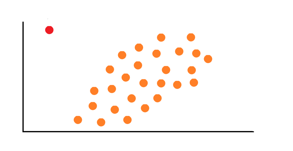
Global outliers 

Global outliers or points anomalies are data points that deviate strongly from the rest of the points. If you plot them it would come to you as quite “obvious”. Most, if not all, outliers detection techniques attempt to identify global outliers. 

An example of global outliers could be a very large order received in a day or a spike in a time series.

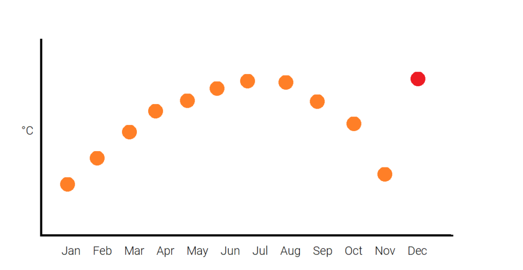
Contextual outliers

Contextual outliers, also called conditional outliers, are extreme observations that deviate from the rest of the observations based on a specific condition (context). Consequently, a reason has to be given as to classify these as outliers. Let’s assume we have a 35°C temperature in London during winter (December). 35°C, by itself, is not an outlier since it’s a common temperature during summer or in the southern hemisphere in December.  

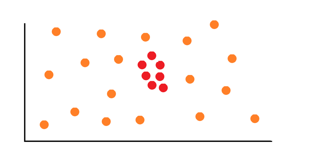
Collective outliers

Collective outliers are a subset of observations whose values as a group deviate significantly from the rest of the observations. However, their individual value might not differ far from the rest o the observations.

For example, if you look at individual device electrical output, you might not see extreme values. However, if you cluster them by location, you see a group of devices closely grouped which increases the electrical output in one location, then that may be an outlier.

Detect outliers with Python [5 methods]

There are many strategies when it comes to detecting outliers. Let us first set up the dataset for outlier detection. For this task, we will use the Boston dataset. Let’s import the data and plot the categorical variables. Looking at the categorical features, we can see from the box plot that the CRIM (Crime per Capita) and the ZN (proportion of residential land zoned for lots over 25,000 sq.ft.) have a lot of points outside 1.5*IQR. Looking at the column from a univariate perspective, one can say that they may be outliers. From now on, let’s apply the outliers detection technique to the CRIM variable.

# Load libraries
import numpy as np
import pandas as pd
import matplotlib.pyplot as plt
import seaborn as sns
from scipy import stats
from sklearn.covariance import EllipticEnvelope
from sklearn.datasets import load_boston


#Load data
boston_data = load_boston()

#Create data frame
df = pd.DataFrame(boston_data.data, columns = boston_data.feature_names)

# Plot boxplot for categorical var
plt.figure(figsize = (14,8))
ax = sns.boxplot(data=df[['CRIM', 'ZN', 'INDUS', 'RM', 'AGE', 
                          'DIS', 'RAD', 'PTRATIO','LSTAT']], 
                 palette="OrRd", )
ax.set_xlabel('Categorical variables')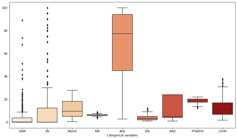

1- Standard Deviation outlier detection method

The first method is a very simple one that you can use to quickly get rid of extreme value. It is not the most robust one, but if outliers but is much simpler to implement than the other methods.

Here, an outlier is defined as a data point that is two standard deviations away from the mean. 

# Standard deviation method
def mark_outliers_2STD(feature):
    std = np.std(feature)
    # Lower end
    le = np.mean(feature) -  (2*std)
    # Upper end
    up = np.mean(feature) + (2*std)
    # Result 
    return [1 if value >= up or value<= le else 0 for value in feature]

# mark outliers
res = mark_outliers_2STD(df.CRIM)

# print number of outliers
print("Number of outliers : ", np.sum(res))

# Add outliers as feature
df["outliers_CRIM"] = res

Number of outliers :  16

2 – Z-score outlier detection method

This technique is slightly more advanced than the previous one used in the sense that you can set the amount of standard deviation away from the mean for the points to be considered as outliers. Here, instead of manually setting the threshold, this method takes advantage of the statistical z-score. 

\mu=\frac{1}{N}\sum_{i=1}^{N} X_{i}

\sigma=\sqrt{\frac{1}{N-1}\sum_{i=1}^{N} (X_{i} - \mu^2)}

For every data point (Xi), we measure how many standard deviation ( \sigma) away from the mean ( \mu ).

Z_{n} = \frac{X_{n} - \mu}{\sigma_{X}}

Naturally, we have to set a threshold for z. Generally, you will see the value 3 to be standard. It is because if a feature is normally distributed, 99.7% of the data points within the features will tend to be located within 3 standard deviations around the mean.  Similar to the previous technique, the z-score outlier detection is meant to be used on a univariate series.

One downfall of using this method is the fact that it is highly sensitive to the mean and the standard deviation which are by themselves sensitive to the outliers. As a result, it decreases the robustness of this method since finding one outlier is dependent on finding the other because every observation tends to affect the mean. Additionally, for optimal use, the underlying distribution of the feature should be normal. 

Taking the previous feature, we can see that this method managed to identify observations as outliers.

def mark_outliers_zscore(feature, threshold = 3):
    # get the z score
    z = np.abs(stats.zscore(feature))
    # return marked value if above threshold 
    return  [1 if value >= threshold  else 0 for value in z]

# mark outliers
res = mark_outliers_zscore(df.CRIM)

# print number of outliers
print("Number of outliers : ", np.sum(res))

# Add outliers as feature
df["outliers_CRIM"] = res

Number of outliers :  8

3- Tukey’s box plot 

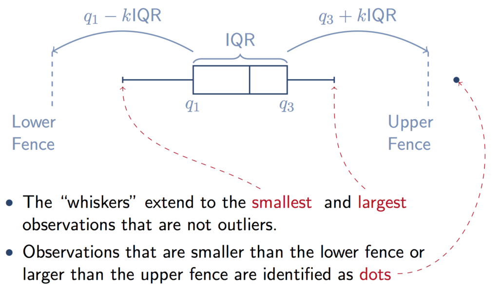
This is a more visual way to detect outliers. See the box plot we used to identify what feature may have a lot of outliers? We are simply going to translate that plot into code and use the statistical concept behind that plot to extract the outliers. If you know how to read a boxplot, then understanding how this works should not be a problem.

One advantage of using this technique is the ability to distinguish between potential outliers and definite outliers (almost definite since one can never be 100% sure). Looking at the table, a probable outlier would be a data point situated between the outer and inner fence. A definite outlier, on the other hand, would be located outside the outer fence.

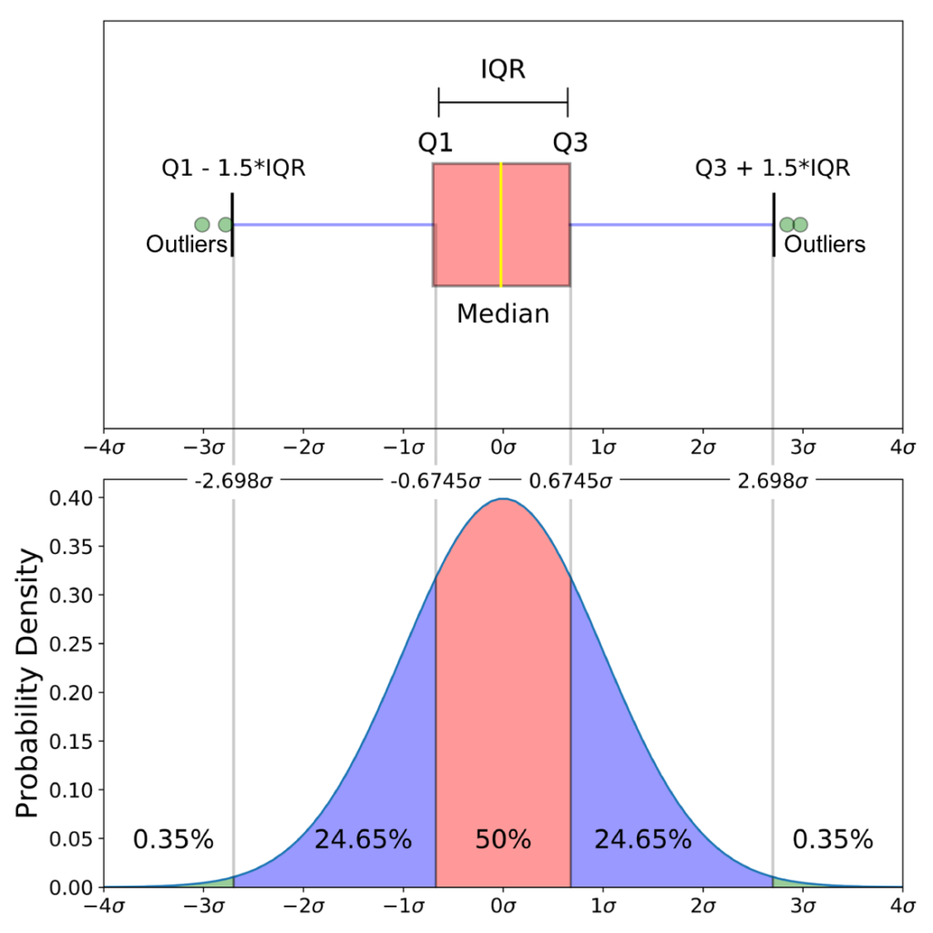
Tukey’s boxplot slightly differs from your standard box plots because the inner and outer fences are not shown. However, we can easily calculate them using the interquartile range (IQR).

The inner fence would be set 1.5 x IQR below Quartile 1 (Q1) and 1.5 x IQR above Q3. The outer fence, however, would be set at 3 x IQR below Q1 and 3 x IQR above Q3. The full calculation can be represented below:

 Q3 = 75th quartile and Q1 := 25th quartile

IQR =Q3 – Q1

Inner fence = [Q1-1.5*IQR, Q3+1.5*IQR]

Outer fence = [Q1–3*IQR, Q3+3*IQR]

Here’s the python implementation of Tukey’s boxplot

#Tukey's method outlier detection
def mark_outliers_tukeys_methodology(feature):
    # get the points statistics
    q1 = np.quantile(feature, 0.25)
    q3 = np.quantile(feature, 0.75)
    iqr = q3-q1
    i_f =  1.5 * iqr
    o_f = 3 * iqr
    
    # Get the outer fence upper and lower end
    # Outer Fence Upper End
    o_f_u_e = q3 + o_f
    # Outer Fence Lower End
    o_f_l_e = q1 - o_f
    
    # Get the inner fence upper and lower end 
    # Innter Fence Upper End
    i_f_u_e = q3 + i_f
    # Inner Fence Lower End
    i_f_l_e = q1 - i_f
    
    definite_outliers = []
    potential_outliers = []
    for value in feature:
        if value <= o_f_l_e or value >= o_f_u_e:
            definite_outliers.append(1)
        else: definite_outliers.append(0)
        
        if value <= i_f_l_e or value >= i_f_u_e:
            potential_outliers.append(1)
        else: potential_outliers.append(0) 
    
    return definite_outliers, potential_outliers

#Extract outliers    
def_outliers, pot_outliers = mark_outliers_tukeys_methodology(df.CRIM)

# print number of outliers
print("Number of outliers : ", np.sum(def_outliers))
print("Number of outliers (potential) : ", np.sum(pot_outliers))

# Add outliers as feature
df["outliers_CRIM"] = def_outliers
df["outliers_CRIM_POT"] = pot_outliers

Number of outliers :  30
Number of outliers (potential) :  66

The Tukey box method is great because it is a very robust method, comparing them to the previous two. It is because the underlying statistical measures used are independent of all other outliers. Besides being quick to calculate, this method does not require the underlying distribution of the feature to be normal. This means that this technique can accommodate a lot of real-life examples. To make this method even more robust, calculate the log of each value before getting the inner and outer fence. The log method of Tukey’s box plot is called the log-IQ method.

The Tukey’s box plot is used on a univariate distribution.  

4- Median Absolute Deviation outlier detection

Robustness, as you may notice, is very important when it comes to outliers detection. The idea behind Median Absolute Deviation is to replace the mean and the standard deviation with more robust statistical measures, such as the median and the median absolute deviation.

MAD = median(|X_i - \mu |)

The test statistic and the identification of outliers work similarly to the z score method where the threshold is set 3 standard deviations away from the median. The MAD above is used in a univariate setting.

def mark_outliers_MAD(feature):
    median = np.median(feature)
    mad = np.abs(stats.median_abs_deviation(feature))
    thres = 3
    return [1 if (((value - median) / mad)>thres) else 0 for value in feature]

# mark outliers
res = mark_outliers_MAD(df.CRIM)

# print number of outliers
print("Number of outliers : ", np.sum(def_outliers))

# Add outliers as feature
df["outliers_CRIM"] = res

Number of outliers :  30

5 – Elliptic Enveloppe method

The basic idea of the Elliptic Envelope method is to draw an ellipse around the data. The data points within the ellipse are doing to be your normal data points and the ones outside it are going to be your outliers. The quite simple technique is very easily implementable.

The two major drawbacks of the Elliptic Envoloppe are, for a better performance the data has to be normally distributed and that we are supposed to set a contamination value. The contamination value tells you the proportion of your observations that are outliers, which we inherently do not know.

def mark_outliers_elliptic_envelope(data, reshape = False, 
contamination = .1):
    if reshape == True:
        data = np.array(data).reshape(-1, 1)
    
    # initialize the Elliptic Envelope
    ee = EllipticEnvelope(contamination=contamination)
    
    # Fit the Elliptic Envelope to the data
    ee.fit(data)
    
    # Predict the outliers  outliers
    return [0 if value == -1 else 1 for value in ee.predict(data)]


# mark outliers
res = mark_outliers_elliptic_envelope(df.CRIM, True)

# print number of outliers
print("Number of outliers : ", len(res) - np.sum(res))


# Add outliers as feature
df["outliers_CRIM"] = res

Number of outliers :  51

6- Mahalanobis Distance method

The Mahalanobis Distance is a widely used technique for outliers detection especially when it comes to contextual outlier detection. The idea behind this technique is to measure the distance between data points and distribution. In a nutshell, the MD defines how many standard deviations a point x is away from the mean of a distribution D. It is represented by 

MD_n = \sqrt{(x_n - \hat{\mu}_X)C^{-1}(x_n -\hat{\mu}_X )^T}

where x represents a vector of observation, \mu the arithmetic mean vector of the columns (independent variables) in the sample, C(-1) is the inverse covariance matrix of the columns. 

Each observation will be compared to a threshold. If we assume a set of features (columns) normally distributed with k features, the Mahalanobis distance will follow a chi-square distribution with K degrees of freedom. You can then set the significance level of your threshold value at (2.5, 1, 0.01). This threshold is defined as:

c = \sqrt{\chi^{2}_{K},q}

One disadvantage of using this method is the fact that the mean and the covariance are highly sensitive to outliers in the data, hence decreasing its robustness. The next method, based on the Rousseuuw determinant method, creates a more robust estimate for \mu and C.

def mark_outliers_mahalanobis(data):
    x_minus_mu = data - np.mean(data)
    cov = np.cov(data.values.T)                           
    inv_covmat = sp.linalg.inv(cov)                  
    left_term = np.dot(x_minus_mu, inv_covmat) 
    mahal = np.dot(left_term, x_minus_mu.T)
    matrix = np.sqrt(mahal.diagonal())

    outlier = []
     #df (degree of freedom) = number of variables
    C = np.sqrt(chi2.ppf((1-0.001), df=data.shape[1]))   
    
    return [1 if value > C else 0 for value in matrix]
    

df["outliers"] = mark_outliers_mahalanobis(df[["DIS", "INDUS"]])
ax = sns.scatterplot(x="INDUS", y="DIS", data=df,hue ="outliers" ,
palette= "OrRd")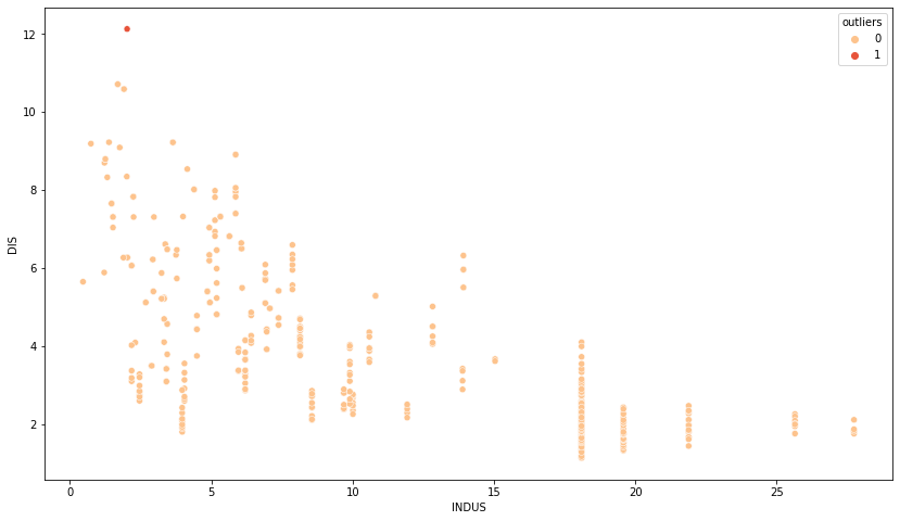

7- Robust Mahalanobis Distance method

The robust Mahalanobis distance introduces the Minimum Covariance Determinant that provides a more robust estimate for \mu and C. It does so by using only the data points of the smallest determinant of the covariance matrix. It is represented by the following formula.

RMD_n = \sqrt{(x_n - \hat{\mu}_{R,X})C^{-1}_{R}(x_n -\hat{\mu}_{X,R})^T }

def mark_outliers_robust_mahalanobis(data):
    seed = np.random.RandomState(8)
    original_covariance = np.cov(data.values.T)
    dist = seed.multivariate_normal(mean=np.mean(data, axis=0), 
                                 cov=original_covariance, 
                                 size=data.shape[0])
    
    cov = MinCovDet(random_state=0).fit(dist)
    mcd = cov.covariance
    robust_mean = cov.location_  
    
    x_minus_mu = data - robust_mean
    inv_covmat = sp.linalg.inv(mcd) 
    left_term = np.dot(x_minus_mu, inv_covmat)
    mahal = np.dot(left_term, x_minus_mu.T)
    matrix = np.sqrt(mahal.diagonal()) 
    outlier = []
    C = np.sqrt(chi2.ppf((1-0.001), df=data.shape[1]))   
    
    return [1 if value > C else 0 for value in matrix]



plt.figure(figsize = (14,8))
df["outliers"] = mark_outliers_robust_mahalanobis(df[["DIS", "INDUS"]])
ax = sns.scatterplot(x="INDUS", y="DIS", data=df,hue ="outliers" ,
palette= "OrRd")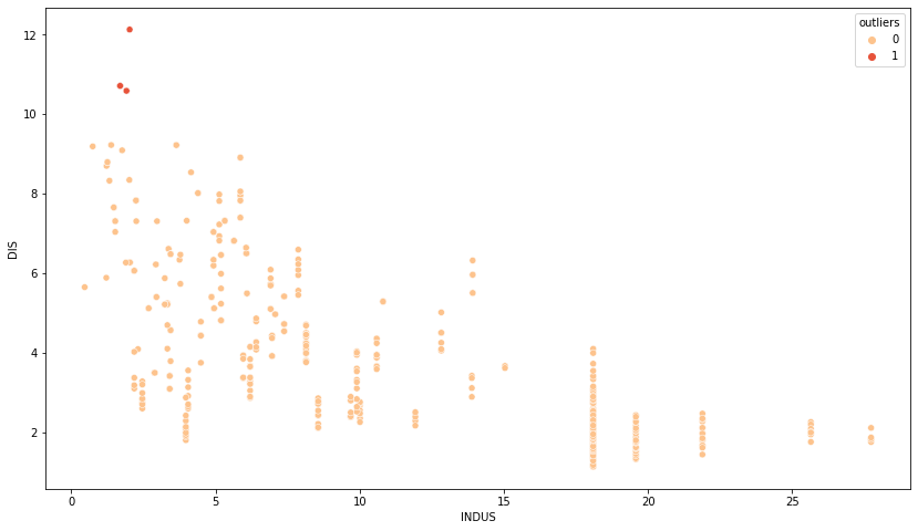

The robust Mahalanobis methods will then pick up slightly more outliers than the standard Mahalanobis method.

Handle Outliers with Python [4 methods]

When we talk about handing outliers in data mining, you have to think about how you can effectively remove them/not include them without necessarily losing too much informational value. What do I mean by data? When we identify outliers with the techniques mentioned above, we are essentially saying that this record should not be considered. It may happen though that the outlier is part of a set of features (columns). It may be an outlier in one column but is not an outlier in the rest of the columns. Ergo, if we remove it, we may end up losing the information it holds in the rest of the feature. 

Based on the type of your project, there are four ways I can think of when it comes to handling outliers. 

1- Mark them

Marking outliers is the easiest method to deal with outliers in data mining. Indeed, marking an outlier allow you to let the machine know that a point is an outlier without necessarily losing any informational values. That means that we are likely not going to delete the whole row completely. 

Using this technique allow us to analyze the outliers to see if they had an effect. The inconvenience of simply marking is that it makes the data set more complicated than it needs to. I mean we are adding new features to the data.

For all the above examples, I have been marking the outliers. I did it by saving the outliers in an array of 0 and 1, with 0 = not outlier and 1 = outlier. Then I appended said array to the data dataframe.

2- Replace them 

Another way of dealing with outliers in data mining is simply replacing them with one of the point statistics. Mean, Median, Q1|Q3, mode, etc. 

Replacing outliers with point statistics can create a lot of bias in your data, especially if you have a lot of them. However, using this technique means that there is minimal information loss and no additional features added.

3- Remove them 

Dropping outliers is yet another way to handle outliers in data mining. It should not be your go-to way of handling outliers since you will lose so much information in the data if you drop every outlier you encounter.

Generally, you should drop the outliers that are due to an error in measurement (40C in the North Pole)/ mistake, or create a relationship that should not be there (eg. 1 red ball amongst 99 green balls). Then you can drop them. In any other case, you can still drop them, but it is advisable to leave a note on dropping those points and how dropping them affected the results.

4- Rescale them 

Another option to deal with outliers is to rescale them. Decreasing the range does decrease the impact of the outliers.

Besides using log or square root transformations, you can take advantage of the robust scalers to reduce outlier’s impact on your models. Indeed, the standard standardization algorithm is sensitive to outliers since its formula ( x’ = (X – mean) / standard deviation. The mean is not as robust to outliers than the meadian. The robust data scaler takes advantage of the robust meadian and the IQR to rescale the data. In here., X’ = (X – median) / (Q3 – Q1)

As a result, we will have a distribution with a mean of 0 and a standard deviation of 1. This is great because the distribution will not be skewed by outliers and the latter will still have approximatively the same relationship as before the data transformation.

Why is handling outliers important?

When doing the exploratory data analysis for a project, there is a lot of assumption we make about the shape and behavior of a population. Having outliers within our data can have a significant impact on the conclusion we derive from the data model. For example, if you have a population of 5 people who have all the age of 30, the average age of the said population will be 30. If you then add someone who is 90 years old, the average age of that population is 40. But, if we look at the individuals within that population, we know that all but one is above 30. As a result, concluding that the average age of that population is 40 might not be the best representation of that population. Consequently, we would handle the individual who is 90 differently, with the techniques mentioned above, to have a more cohesive understanding of our data and to draw more realistic conclusions.

Outliers are not only appearing because of the characteristics of the data, they can be due to human error as well. So, handling outliers can reveal issues in the data collection process. Those types of mistakes are called error-outliers and need handling. 

Last but not least, detecting and handling outliers in data mining tend to improve your machine learning models. if you think of machine learning models as mathematical algorithms that make a prediction based on the provided data, you will have the wrong prediction if the data you start with is bad. My bad, I mean that the data is not representative of the true population. Therefore, handling outliers in your ML models can lead to better results.

Sources

https://www.machinelearningplus.com/statistics/mahalanobis-distance/

https://towardsdatascience.com/detecting-and-treating-outliers-in-python-3a3319ec2c33

http://www.hermanaguinis.com/ORMoutliers.pdf

https://www.sciencedirect.com/science/article/abs/pii/S0022103117302123